Mandelbrot Set Rendering

1 Introduction

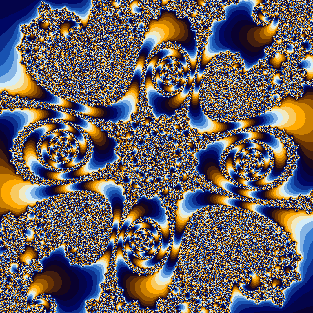
Recently I read ”Fractal Programming in C” by Roger T. Stevens[6]. A fractal is, as Stevens writes ”a curve whose Hausdorff-Besicovitch dimension is larger than its Euclidean dimension”. A more informal definition would be that a fractal is, as I write, ”an infinitely complex shape which is self-similar across arbitrarily small scales”. Stevens describes over a dozen different kinds of fractals, including example source code to render each one. Additionally, Stevens provides several full color prints of his favorite renders. These renders disproportionately feature incrementally smaller scaled renders of the Mandelbrot set. I had some familiarity with the Mandelbrot set and found these renders striking. Thus I took it upon myself to write my own renderer inspired by Stevens.

I began with an implementation like Stevens describes. It was single-threaded, direct, and very slow. Rendering a 4k image took minutes even at modest iteration counts, and particularly small scales or ”deep zooms” were impossible. I spent about two months studying and implementing the techniques used in the most advanced fractal renderers: arbitrary floating point arithmetic, numerical techniques such as linear approximation and perturbation theory, non-standard floating point types, and parallelism on both the CPU and the GPU. By the end of that process, my renderer could perform the same 4k render it struggled with before in milliseconds, achieving arbitrarily deep zooms.

This document describes that renderer in a step-by-step manner. It starts from the naive implementation, and builds up to the complete version, detailing the theory and practice of each improvement.

2 Fundamentals

Let \(\mathbb {C}\) represent the set of all complex numbers. The Mandelbrot set \(\mathbb {M}\) is the set of \(c\in \mathbb {C}\) such that the recursively defined sequence \(z_{n+1} = z_n^2 + c\) with \(z_0 = 0\) does not diverge to infinity. The sequence \(z\) is often called an ”orbit”, because each iteration rotates and scales the complex plane (via \(z^2\)) and then translates it (via \(+c\)).

Suppose there is an image \(I\) with \(I_\textrm {width}\) and \(I_\textrm {height}\). Let pixel coordinates in \(I\) be

To render \(I\), each \(p\in \mathbb {P}\) must be assigned some \(v\in \mathbb {V}\) where \(\mathbb {V}\) is the set of all color values. From these definitions, it can be said that writing a renderer is to define some rendering function \(f:\mathbb {P}\rightarrow \mathbb {V}\). Consider writing a renderer for \(\mathbb {M}\). It can be inferred from \(\mathbb {M}\subset \mathbb {C}\) that there must be some composition such that \(f = f_2:\mathbb {C} \rightarrow \mathbb {V} \circ f_1:\mathbb {P} \rightarrow \mathbb {C}\).

\(f_1\) is trivial to define. Notice that elements of \(\mathbb {P}\) and \(\mathbb {C}\) have the same number of components: x and y for \(P\), real \(\Re \) and imaginary \(\Im \) for \(\mathbb {C}\). Thus we can construct the mapping \((p\in \mathbb {P})\leftrightarrow (p_x + ip_y)\in \mathbb {C}\). However, when plotting, we generally want to have control over the view port. The view port can be defined as two complex numbers \(c\) and \(s\) representing the corner and size of the view port respectively. We can say that

\(f_2\) is more difficult to define. The most common definition is using the ”escape time” algorithm. It goes something like this: Start at \(z_0\) with \(n=0\). Iterate until either \(|z_n| > r\) for some ”escape radius” \(r\), or \(n = N\) for some maximum iteration count \(N\). The value of \(n\) gives us an idea of whether \(c\) is in \(\mathbb {M}\). If the orbit escapes before the maximum iteration count, i.e. \(n < N\), then \(c \notin \mathbb {M}\), because we observed \(z_n\) diverge. We cannot know for certain that \(n = N \Rightarrow c \in \mathbb {M}\), because continuing to iterate might eventually reveal divergence; we are approximating. Let \(f_N:\mathbb {C}\rightarrow \mathbb {N}\) be the escape-time function. Notice that we still need to derive an element of \(\mathbb {V}\) to satisfy our definition of \(f_2\). Let \(f_v:\mathbb {N}\rightarrow \mathbb {V}\) such that

. Naively we may say

Notice that most of the information about \(n\) is lost. All escape times in the arbitrarily large interval \([0, N)\) are represented without differentiation.

Note that the special case for \(n=N\) is preserved such that regardless of \(N\) the color of pixels with \(c\in \mathbb {M}\) can be explicitly defined.

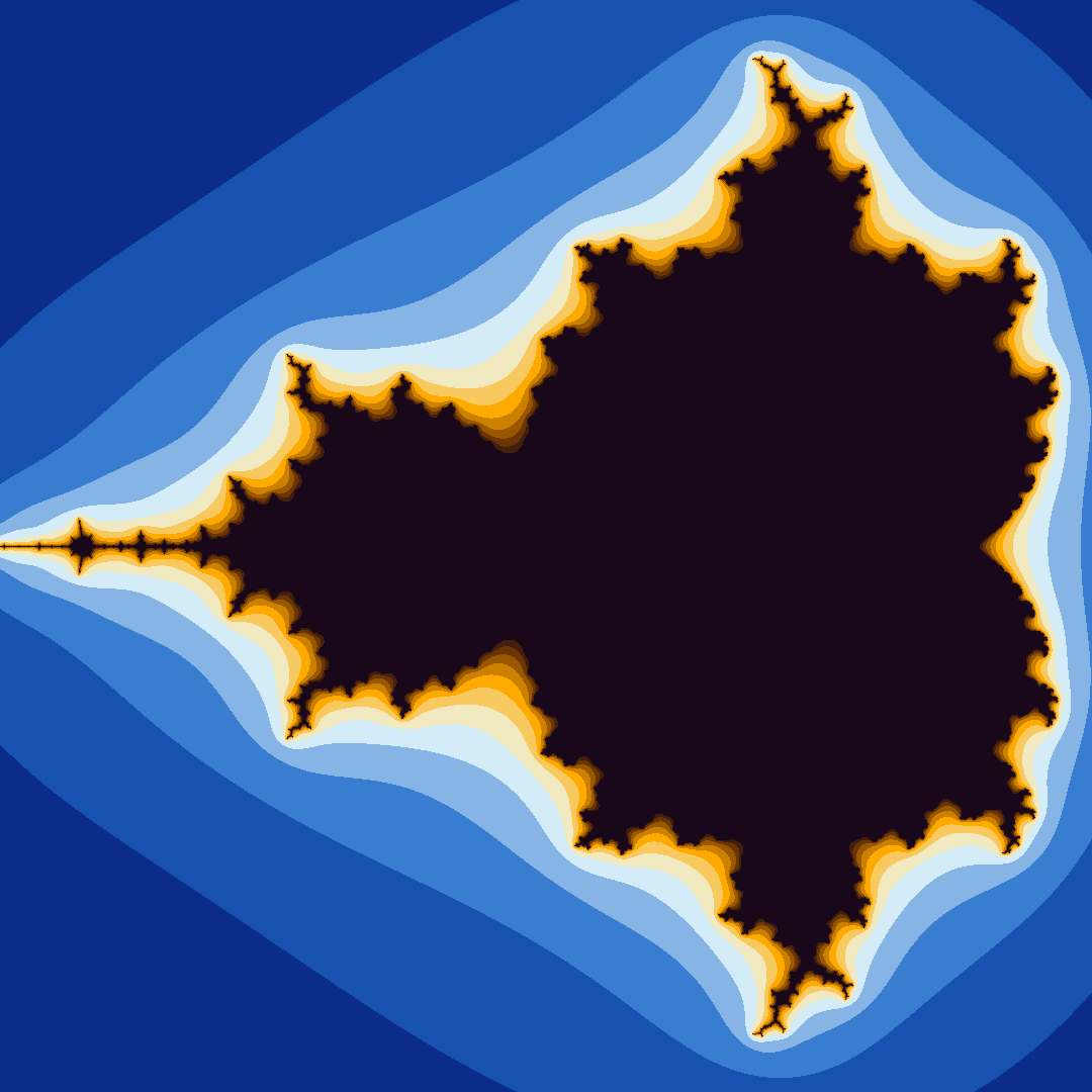
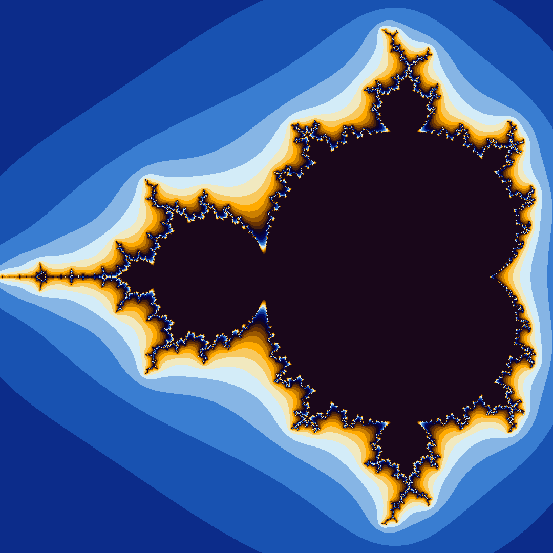
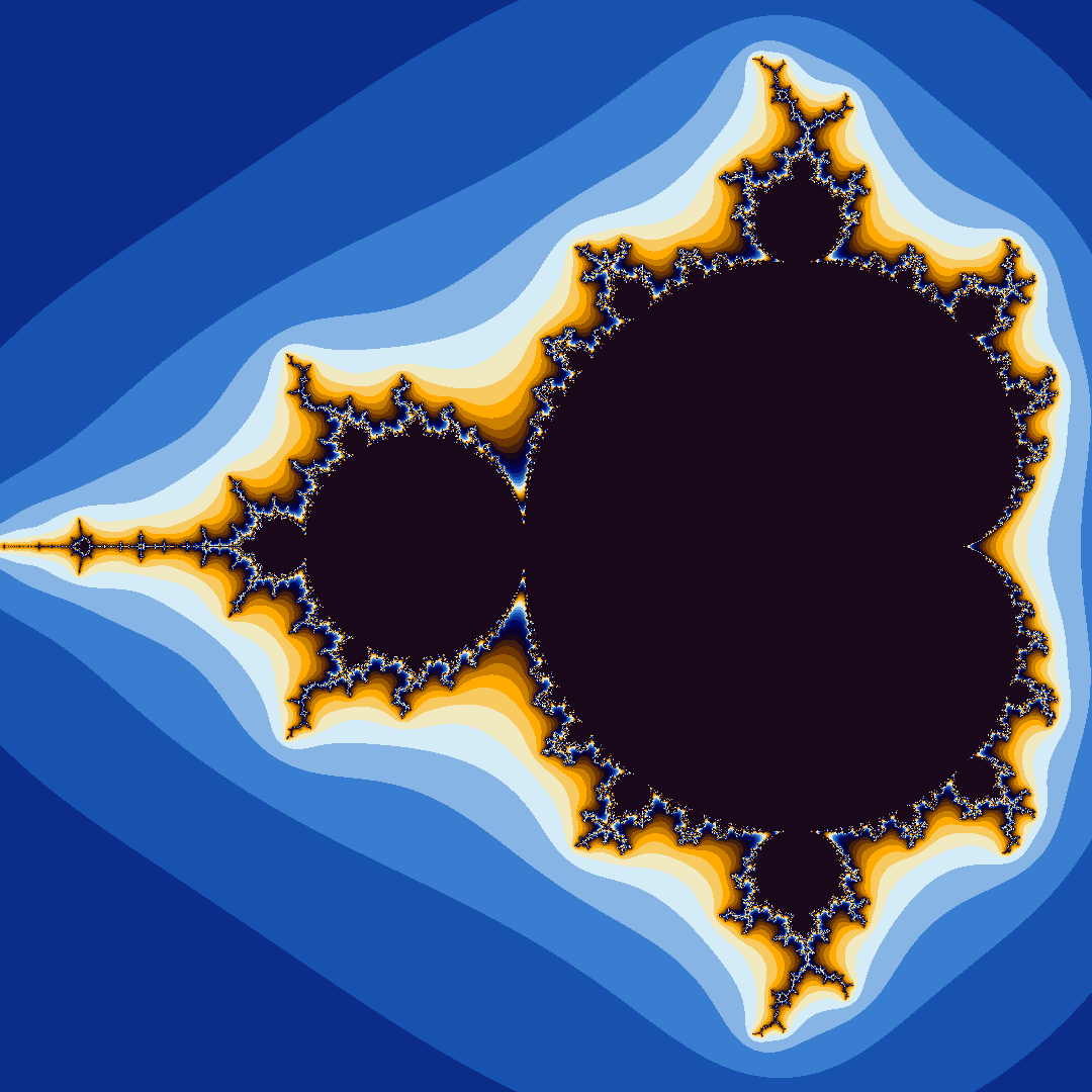
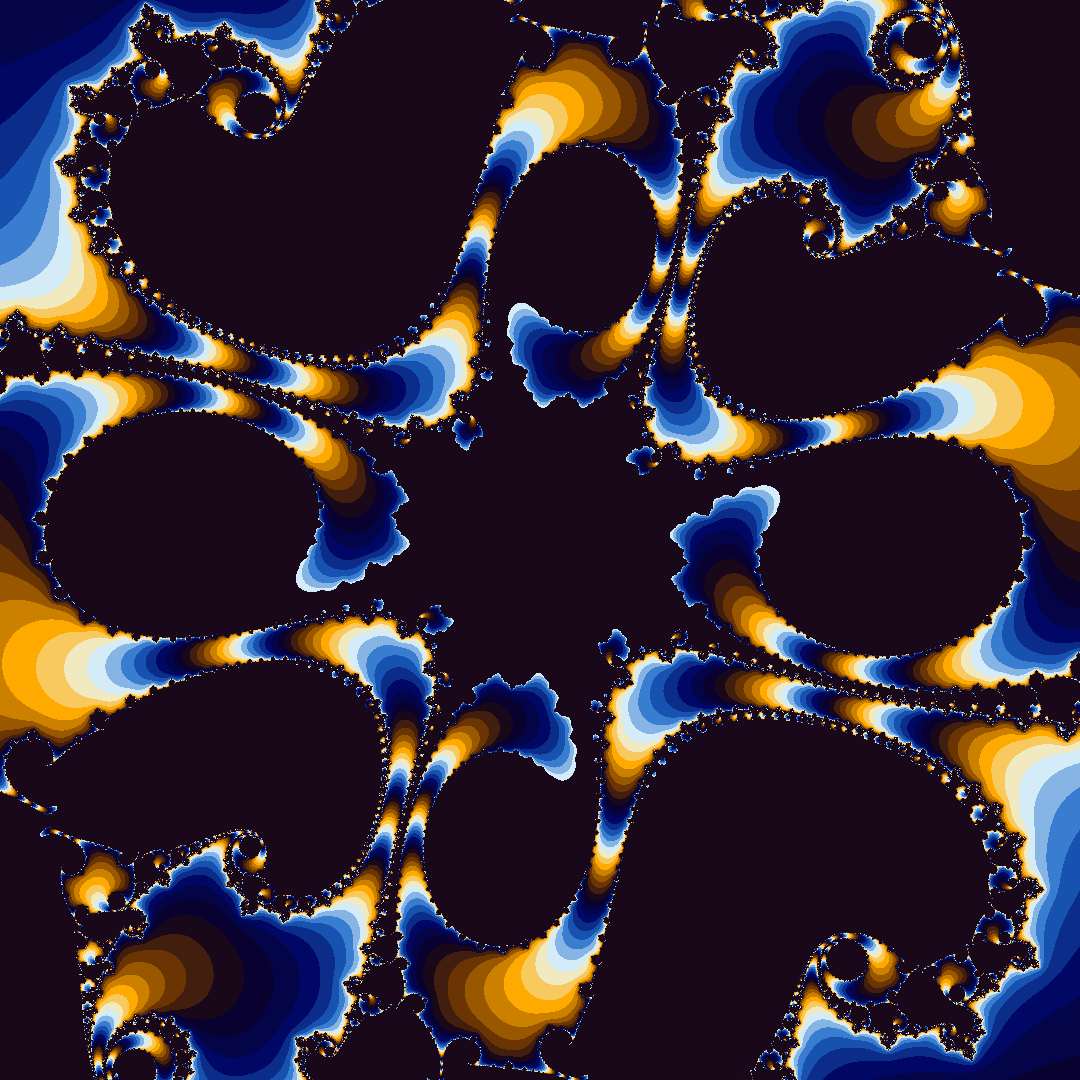
The larger the value of N the more detailed and accurate the render will be. See Figure 1 and Figure 2.

2.1 Continuous Coloring

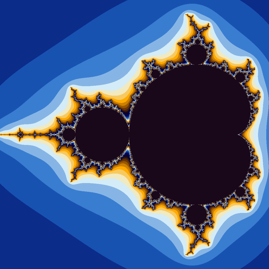
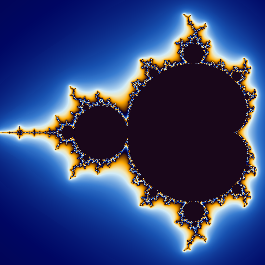
In the above renders you may have noticed the harsh color banding. Stevens’s renders had the same property. This follows naturally considering escape time is a discrete value. To achieve smooth coloring, the continuous value of our orbit \(z_n\) must be used. It has been approximated that

\(n_{\textrm {cont}}\) can be used to linearly interpolate between \(f_v(\lfloor n_{\textrm {cont}} \rfloor )\) and \(f_v(\lceil n_{\textrm {cont}} \rceil )\). The derivation of \(n_{\textrm {cont}}\) is well explained by Dr. Linas Vepstas[8]. I have little to add to it so I will not summarize that explanation here.

Observe the differences between continuous and discrete coloring algorithms in Figure 3.

3 Arbitrary Precision

Fixed precision is the default for floating point arithmetic. There are two standard floating point types: a single precision type (a ”float” in C-terms) stored in 32 bits, and a double precision type stored in 64 bits (”double” in C-terms). As our view port gets smaller, we may lose the precision required to adequately differentiate between pixels.

We can go much further if we instead use arbitrary precision. Arbitrary precision is the storage of floating point numbers with arbitrary size, typically dynamically allocated like a list (or a vector, if you prefer). The GNU MPFR library offers this for floating point numbers and is commonly used in scientific computing, giving us theoretically infinite precision, bounded only by our hardware.

However, we quickly encounter practical hardware limitations. Arithmetic with arbitrary precision numbers is horribly slow compared to fixed precision. What looks like one operation with arbitrarily sized numbers is implemented as arbitrarily many fixed size operations. Further, renders that require greater precision also require greater iteration counts, exacerbating the performance cost of these kinds of calculations.

4 Perturbation Theory

4.1 Basics

Claude Heiland-Allen showed that ”if you have two high precision numbers close together, their difference has less meaningful precision”:

[4]

Perturbation theory relies on this fact. The idea is that one high precision orbit is stored as a reference. The escape time of nearby orbits is calculated using their differences from the reference orbit.

Let \(Z\) be the reference orbit. Let \(C=Z_0\). Let \(z\) be another orbit with \(c=z_0\). Let \(\Delta z_n = z_n - Z_n\). K.I. Martin showed that from these definitions it can be derived:

[5] Martin notes that ”all the numbers are ’small’, allowing it [perturbed orbits] to be calculated with hardware floating point numbers”. This is important because the reference orbit can be computed with arbitrary precision when necessary, while the speed of fixed precision can be leveraged for the bulk of computations.

4.2 Glitches

When \(|\Delta z|\) becomes too large the escape time of the \(z\) calculated with perturbation diverges from the true escape time of \(z\). This creates visual ”glitches” of large groups of nearby pixels incorrectly being assigned the same color. Some early solutions to this included doing a pass over the resulting image to detect glitches, and recoloring them required using a closer reference orbit. However, there is a method which requires no additional reference calculations.

Rebasing is a technique to avoid glitches. The idea is that as we iterate \(\Delta z\), if it drifts from the reference we restart the reference iteration and assign \(z_n\) to \(\Delta z_n\). The validity of this method relies on multiplication of complex numbers representing a rotation[9]. A perturbed sequence using rebasing can be defined mathematically likewise:

5 FloatExp

While perturbation theory allows us to stretch our fixed precision numbers further, we still reach a point where we lack the precision to adequately represent the delta from an orbit to the reference without underflow. For doubles this is at a zoom factor of \(\sim 10^{-308}\). Arbitrary precision would solve this, but at that point there is no benefit to using perturbation theory. A more precise fixed size floating point type is necessary.

Some languages and libraries offer a quad, which uses 128 bits. A quad offers a larger exponent and mantissa. However, as the viewport gets smaller, the relative difference between pixels stays constant. This means that while the renderer could make use of the larger exponent, the larger mantissa will remain unused, making a quad inefficient for our use case.

”FloatExp” is a type which joins a hardware floating point type and an integer which represents its exponent. This will make more efficient use of memory than the quad, while allowing zooms to go much deeper than a double or a float. Performing arithmetic with these numbers is more complicated and computationally intensive. Binary operations on the floating point components require the integer components to be equal. As such, one operand must adjust its integer component by some \(x\) to match the other, multiplying its floating point component by \(10^{-x}\) to preserve its value. This multiplies the number of required operations substantially. However, this cost is preferable to the alternatives: being unable to render at all, using an inefficient and similarly expensive quad type, or using much slower arbitrary precision.[3]

6 Bivariate Linear Approximation

With good approximations we can produce almost visually identical renders substantially faster. Taylor Series Approximations were once regarded as the best option for this, but now consensus is that the bivariate linear approximation (BLA) is superior.

Recall the perturbation formula:

[7] BLA takes advantage of the fact that if \(\Delta z_n^2\) is small enough it will have no effect on \(\Delta z_{n+1}\) and we can instead write the linear equation:

Because this equation is linear, we can combine many iterations into one computation:

[7]

Determining if we can use a given BLA to skip from \(m\) to \(n\) is a matter of determining if the squared term \(\Delta z_n^2\) is ”small enough” to ignore. ”Smallness” is relative to the other terms of the equation. Thus, it can be said some BLA is valid if

This validity check will be performed each escape time iteration with each candidate BLA, so it is worth reducing the computations required as much as possible. Both sides can be divided by \(\Delta z_n\).

The coefficient of \(Z_n\) can be moved into \(\varepsilon \)

Since

We can substitute

And isolate \(\Delta z_m\)

[7] Note that every value on the right side of the equation other than \(\Delta c\) is independent of the orbit for which the BLA’s validity is being checked. If the maximum possible value for \(\Delta c\) is used, the right side of the equation can be computed once for all validity checks of which there may be several trillion in a render. Let

where \(r\) is the validity radius of a BLA.

Ideally, there would be BLAs from every possible value of \(m\) for every possible value of \(l\). However, that would mean calculating \(O(n^2)\) BLAs, which is an alarming time complexity that likely does not amortize its cost. There is an alternative approach which is faster and retains most coverage. First, all single iteration BLAs are computed. Then, each sequential pair is combined following Claude’s BLA merging formulas[2]. Repeat until no longer possible. This creates a binary tree of BLAs in \(O(n)\) time complexity.

Faster escape time computations can be performed using BLAs. Each iteration, check the BLAs with \(m=n\). If the lowest-level BLA is invalid, then no other BLA can be valid, and we continue with a normal perturbation iteration. Otherwise, search from the highest-level down for the first valid BLA, as it will allow the renderer to skip the most iterations. Repeat until the escape condition is met[7].

7 Zoom Video Rendering

So far we have only discussed the rendering of single images and alluded to video rendering. Note that when I refer to video rendering, I am specifically referring to zoom videos, videos of zooming progressively deeper into a specific point in the complex plane. Videos of this sort are aesthetically pleasing and show the chaotic properties of fractals such as \(\mathbb {M}\).

We need to know how many frames to render. Let \(F\in \mathbb {N}\) where \(F\) is the total number of frames in our video. There are many ways to determine \(F\) depending on how we want to describe our video. I wanted to be able to express a beginning and ending view size \(a\) and \(b\), a frame rate \(s\), and a factor \(z\) by which the view size changes every second. It is trivial to represent the relationship between these variables and then isolate \(F\).

Each frame must have a view port \(V\) with components \(V_{\textrm {center}}\in \mathbb {C}\) and \(V_{\textrm {size}}\in \mathbb {C}\). Since the center point will always be the focus of the zoom, \(V_{\textrm {center}}\) is constant. \(V_{\textrm {size}}\) can be determined by linearly interpolating between \(a\) and \(b\) using the index of the current frame \(f\in [0, F)\).

7.1 Parameters

When rendering a single image parameters can be manually tuned until satisfied with output and render speed. Video renders are composed of potentially thousands of frames, thus heuristics to produce adequate parameters must be derived. These heuristics may be composed using constants which can be tuned manually per video rather than per frame.

For our arbitrary precision numbers we have to specify some number of decimal digits \(d\) which storage should be allocated for. While far from a robust heuristic, I experimentally determined the following heuristic works well:

Similar to \(d\), \(N\) must grow as \(f\) increases. Similar to \(d\), I use an unproven yet experimentally tested heuristic:

We have described several relevant fixed precision floating point numeric types, which I will list in order of increasing size and processing time: single precision, double precision, and FloatExp which may be defined with any combination of floating point type for the mantissa and integer type for the exponent. We will only be dealing with FloatExp types using a double and a 64-bit integer, as it is the largest which can be easily represented on hardware. We could use smaller types which would make FloatExp faster, but only marginally so, and if we need to use FloatExp it is likely precision is more important than speed. We will call this specification DoubleExp or more tersely ”dexp”, and we will not consider other specifications. I mention all this because when we perform a render we will need to select a numeric type. Let the set \(\mathbb {T}=\{\textrm {float}, \textrm {double}, \textrm {dexp}\}\), from which the render’s numeric type will be selected.

We have described three rendering algorithms: direct, perturbed, and approximate perturbed rendering using BLA. Let \(\mathbb {A}\) denote the set of our possible rendering options:

Similar to \(\mathbb {T}\), elements of \(\mathbb {A}\) have different performance costs. direct is always faster than perturbed when using the same \(t\in \mathbb {T}\). approximate can be faster than perturbed, but incurs a cost calculating approximations which may not be made up for by the number of iterations it allows the renderer to skip. Thus perturbed can be faster depending on the location and the iteration counts, usually performing better when iteration counts are under some threshold.

With the definitions of \(\mathbb {T}\) and \(\mathbb {A}\) out of the way, we can consider how we will select optimal \(a\in \mathbb {A}\) and \(t\in \mathbb {T}\) to use for the frame of index \(f\). However, before doing so we need to define some rather complicated \(P(a,t)\) representing the validity of \(a\) and \(t\) for the current frame.

First select \(a\). Experimentally it seems numeric type is much more important than render type in terms of performance. For that reason, because perturbed rendering lets us use a smaller numeric type, direct rendering is only faster when it can be used with a float type. Approximate rendering is significantly faster than perturbed rendering with high enough iterations at most locations. Heuristically, it seems iteration count is the defining characteristic so we can define some threshold for significant iterations \(S\). Define \(a\) like so:

Then it is trivial to select \(t\). Simply choose the smallest valid type:

Suppose that we select an approximate rendering algorithm. The deciding parameter on the validity of an approximation for a location is its ”smallest factor” \(\varepsilon \). The size of \(\varepsilon \) is proportional to the permissiveness of our approximations. Too large, we will have an inaccurate render. Too small and performance will be unnecessarily pessimized. There is not a mathematically provable ideal value of \(\varepsilon \). What can be done instead is we define a range, an upper bound \(\varepsilon _u\) and a lower bound \(\varepsilon _l\) and perform a binary search. To perform a binary search we need to determine if we should assign \(\varepsilon \) to \(\varepsilon _u\) or \(\varepsilon _l\). Let the elements of \(\vec {p}\in \mathbb {C}^n\) be some evenly distributed values (”probes”) in the view port. Let \(\vec {t}\in \mathbb {N}^{n}\) and \(\vec {a}\in \mathbb {N}^{n}\) be the true and approximate escape times for each element of \(\vec {p}\). If \([\exists a,t\in \vec {a},\vec {t}](|\frac {a}{t} - 1| > T)\) where \(T\) is some tolerance for the relative error between \(a\) and \(t\), we can assign \(\varepsilon \) to \(\varepsilon _u\) to shrink the value of \(\varepsilon \). If this is not the case, we assign \(\varepsilon \) to \(\varepsilon _l\) so we can skip more iterations and perform our render faster. We stop our search if \(|\varepsilon _u - \varepsilon _l| < r\) where \(r\in \mathbb {R}\) is some ”convergence radius”. It is worth noting that my renderer does not do precisely this. Instead of performing a binary search for \(\varepsilon \), it performs a binary search on an exponent of base 10 and we use \(\varepsilon =10^{\textrm {exponent}}\) to calculate BLAs.

7.2 Memory

Memory allocations are slow, as are all system calls. Where possible we want to keep execution inside of our program. Consequently, we want to allocate all the memory we will need ahead-of-time. There are two structures we need to allocate memory for: Reference orbits and BLAs.

Since we can calculate the iteration count of the last frame out of order, it is trivial to preallocate all the memory we will need for the reference orbits of each numeric type. Additionally, since we are reusing the same reference orbit between frames, we can also precompute the reference orbit, saving us millions to trillions of unnecessary iterations.

We can similarly use the known iteration count of the last frame to preallocate memory for the maximum possible number of BLAs, as they grow proportionally to the reference orbit length. However, unlike the reference orbits we cannot precompute them. BLAs change from frame to frame, as the \(\Delta c_{\textrm {max}}\) changes as do valid \(\varepsilon \) values. Not only can we not precompute BLAs, but we cannot simply pre-construct the structure and change its values. Depending on the size of the numeric type used for the BLAs, the structure of their memory layout changes. As such, while we initially receive a memory allocation from the system for the BLAs, when it is time to construct them in memory we must allocate the memory ourselves from the buffer we received from the operating system. Because execution remains in our program, these allocations are fast. For this I implemented a linear or ”arena” allocator, which just means that whenever the BLAs needed a piece of memory we allocate it in order and then free all the memory at once when the BLAs are no longer in use.

8 Parallelism

Rendering \(\mathbb {M}\) can be described as ”embarrassingly parallel”. The rendering of each pixel is completely independent, so for almost no extra effort their coloring can be done in parallel. The same can be said for generating BLAs, merging pairs of BLAs, and testing BLA search probes. The renderer becomes much faster just using multiple CPU threads, but the GPU was specifically designed for computer graphics so it ought to be preferred. Most modern CPUs have an integrated graphics chip, so that option should almost always be available.

An algorithm which can less obviously be run in parallel is reference calculation. Reference calculation is performed independently for \(\Re (Z_n)\) and \(\Im (Z_n)\) before the complete \(Z_n\) is stored. Consequently, the calculation of each component can be done in parallel, synchronizing after each iteration for storage. It may occur to you that synchronization overhead would make this slower as computing each component is only a few operations. However, recall that \(Z_n\) is calculated with arbitrary precision before it is cast to fixed precision. Just one operation with arbitrary precision is relatively expensive for the CPU, as it requires many operations to be performed in the fixed precision numbers used to represent it. Thus, the time saved by parallelizing these operations exceeds the synchronization overhead.

Note that if you decide to write a program like this, it is worth considering using a heterogeneous parallel programming API such as SYCL or OpenCL. They allow you to write code which can run in parallel on a variety of CPUs and GPUs. I started out with my own custom abstraction layer, which was an exciting experiment, but adding support for other processors was a considerable effort each time.

9 Other Techniques

There is a lot more that I could have done to optimize or produce more visually interesting renders, but which are beyond the scope of this learning exercise. Still, I would like to yield something from my research, so I have compiled those optimizations and techniques here.

9.1 Distribution

This is effectively an extension of parallelism. In addition to running the renderer in parallel on different threads, it could be easily run in parallel on different machines. The Message Passing Interface (MPI) is standard for this kind of parallel computing. The idea is that some number of processes are spawned across the cluster (group of machines cooperating on some task, linked over a network), with each sharing an environment and communication interface. I imagine that for a \(\mathbb {M}\) rendering cluster we spawn a worker process to manage each GPU, and one process which maintains a queue of frames and distributes them to workers for rendering. Once the queue is empty and the segment is complete, some cooperation is performed to encode that segment and we continue to the next segment until our render is complete. The cluster would have to share a filesystem over the network.

Distributed \(\mathbb {M}\) rendering is largely unexplored. Claude proposed a roadmap for distributed Mandelbrot set rendering in 2013, which, while interesting, went unimplemented[1]. While a pretty major shift in project goals and architecture, if I am to pursue any further optimizations, it is this one. I encourage anyone else who is interested to attempt as well.

9.2 Periodization

We can skip many iterations of \(z\) by leveraging a property of \(\mathbb {M}\). Orbits \(z\) with values of \(c\in \mathbb {M}\) can be said to have a ”period”; their series repeats. If we detect this, we know that \(c\in \mathbb {M}\) and we can skip \(N - n\) iterations where \(n\) is the iteration we detect the period of \(z\). Additionally, for a periodic orbit \(z\) we can find any value in the orbit without computing any additional iterations. That means that if we select a periodic point for our reference \(Z\), then we can abort early, but still have enough references for our pixel orbits. There are mathematical techniques we can apply to find a periodic orbit in \(\mathbb {M}\) bounded by some parameters[7].

References

[1]

Claude Heiland-Allen. A roadmap for distributed Mandelbrot set rendering. Apr. 2013. url: https://mathr.co.uk/blog/2013-04-28_a_roadmap_for_distributed_mandelbrot_set_rendering.html.

[2]

Claude Heiland-Allen. Deep Zoom. May 2024. url: https://mathr.co.uk/web/deep-zoom.html.

[3]

Claude Heiland-Allen. Fast extended range types. url: https://fractalforums.org/programming/11/fast-extended-range-types/4224/msg28686#msg28686.

[4]

Claude Heiland-Allen. Perturbation techniques applied to the Mandelbrot set. Oct. 2013. url: https://mathr.co.uk/mandelbrot/perturbation.pdf.

[5]

K. I. Martin. SuperFractalThing Maths. 2013. url: http://www.science.eclipse.co.uk/sft_maths.pdf.

[6]

Roger T. Stevens. Fractal Programming in C. 1st ed. Redwood City, CA: M&T Books, Aug. 1989.

[7]

Phil Thompson. Faster Mandelbrot set rendering with bla: Bivariate linear approximation. May 2023. url: https://philthompson.me/2023/Faster-Mandelbrot-Set-Rendering-with-BLA-Bivariate-Linear-Approximation.html.

[8]

Linas Vepstas. Renormalizing the Mandelbrot Escape. June 1997. url: https://linas.org/art-gallery/escape/escape.html.

[9]

Zhuoran. Another solution to perturbation glitches. 2021. url: https://fractalforums.org/fractal-mathematics-and-new-theories/28/another-solution-to-perturbation-glitches/4360.